Model Theory
Introduction
WIRM is a modified version of the Streeter-Phelps equation, which is one of the first water quality models originally developed during a study of the Ohio River in the 1920s (Streeter and Phelps, 1925). The model is used to simulate the effect of a Biochemical Oxygen Demand (BOD) point discharge on Dissolved Oxygen (DO) levels of rivers and streams.

Extracted from p. 18 of Streeter and Phelps (1925)
DO and BOD
Dissolved Oxygen
While often thought of as a gas, oxygen readily dissolves into water where it is needed for the survival of various aquatic organisms such as fish. The minimum DO concentration varies by species and organism, but is typically between 4 and 6 mg/L. A number of physical, chemical and biological processes affect the concentration of DO in aquatic ecosystems. DO is consumed by microbial respiration, but also produced by photosynthesis. Gas exchange between the water and the atmosphere also changes the concentration of DO, driving it towards a state of equilibrium. Chemical processes such as deoxygenation can also affect DO levels.
Biochemical Oxygen Demand
Before the invention of modern treatment technologies, wastewater effluent contained high concentrations of organic compounds. When these organic compounds are released in the environment, they are decomposed by microbial organisms and undergo chemical deoxygenation. The total amount of oxygen that is consumed by these processes is referred to as the Biochemical Oxygen Demand (BOD).
The concentration of BOD is often measured by placing a water sample in a dark bottle and measuring the change in dissolved oxygen over time. As the BOD decays, the oxygen is consumed by microbial and chemical processes. The total amount of oxygen that is lost over a specific period of time is then defined as the concentration of BOD. Typically, BOD is measured over a 5-day and referred to as the 5-day BOD (BOD5). The ultimate BOD (UBOD) is the total amount of BOD that would be measured if the experiment were conducted over a very long (effectively infinite) period such that all BOD material is degraded.
Model Interpretation
Before discussing the model equations and parameters, it is useful to understand how to interpret the model output generated by the simulation. Here is an example using the default parameter values:
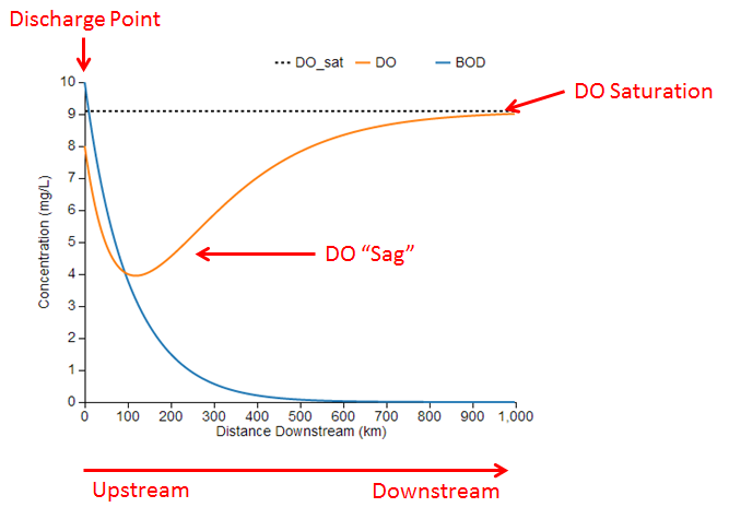
The blue and orange lines represent the simulated concentrations of BOD and DO along a stretch of river. The chart also shows the DO saturation concentration as the dotted black line for reference. These concentrations represent a snapshot of the river at a single point in time.
The left side of the chart (x=0) represents the upstream end of the reach where BOD is being discharged into the river from a point source such as a wastewater treatment plant. Initially, the concentrations of BOD and DO decrease just downstream of the discharge as BOD undergoes microbial decomposition and chemical deoxygenation, which are processes that consume DO.
At some point downstream of the discharge, the DO concentration reaches a minimum value, often called the critical point. At this point, the rates of BOD decay and DO reaeration are balanced because the oxygen lost by BOD decomposition is being replenished by an equivalent amount of oxygen dissolving into the water from the air. Past the critical point, DO increases as the rate of reaeration exceeds the rate of BOD decay and more oxygen is dissolving into the water than is being consumed. Eventually, the BOD has been completely decomposed and its concentration approaches zero. Without any BOD decomposition, the DO level approaches the saturation concentration where it is in equilibrium with the air. The dip in the DO concentration is known as the DO sag, which is a characteristic curve often observed downstream of BOD discharges.
In this example, the minimum DO concentration is about 4 mg/L at a point 120 km downstream of the discharge. If the target minimum DO concentration were 5 mg/L, which is required by some fish species, then we conclude that the BOD concentration is too high to support aquatic life. Using the slider for the initial BOD concentration parameter, L0, we could identify how much the BOD concentration would need to be reduced in order to achieve a minimum DO concentration of 5 mg/L.
Model Schematic
This figure shows a schematic diagram of the model, which includes two state variables: the concentrations of BOD, $L$, and DO, $o$. These variables are subject to two processes: 1) BOD decay, which reduces both BOD and DO, and 2) DO reaeration, which is the exchange of oxygen between the water and air that will increase DO if it is below saturation.

Equations
The model schematic shown above is mathematically represented as a system of two ordinary differential equations (ODEs):
$$\frac{dL}{dt} = -F_{ox}k_dL$$ $$\frac{do}{dt} = -F_{ox}k_dL+k_a(o_s-o)$$where $L$ and $o$ are the concentrations of BOD and DO (mg/L), respectively, $t$ is the downstream travel time (days), $k_d$ is the BOD decay rate (1/d), $k_a$ is the DO reaeration rate (1/d), $o_s$ is the DO saturation concentration (mg/L), and $F_{ox}$ is the BOD/DO inhibition factor (unitless).
Initial Conditions
The equations are solved using the initial concentrations of BOD and DO:
$$L(t=0) = L_0$$ $$o(t=0) = o_0$$These initial concentrations are the in-stream concentrations resulting from complete mixing of the discharge with the river. They can be computed as the flow-weighted mean of the discharge concentration and in-stream concentration just upstream of the discharge point, see below.
Numerical Method
Given the initial concentrations, the differential equations for BOD and DO as a function of travel time are solved using the 4th-order Runge-Kutta numerical method, which is an explicit, forward-stepping scheme.
For a generic variable, $y$, with initial condition $y(t=0)=y_0$ and derivative function $f(t, y)=dy/dt$ the solution for $y(t)$ can be computed incrementally. If $h$ is the step size between each solution point, then:
$$y(t+h) = y(t) + \frac{h}{6}(K_1+K_2+K_3+K_4)$$ where $K_1$, $K_2$, $K_3$, and $K_4$ are defined as: $$ \begin{eqnarray} K_1 & = & f(t, y(t)) \\\ K_2 & = & f(t + h/2, y(t) + h/2\cdot K_1) \\\ K_3 & = & f(t + h/2, y(t) + h/2\cdot K_2) \\\ K_4 & = & f(t + h, y(t) + h\cdot K_3) \end{eqnarray} $$Travel Time and Distance
While the equations above describe the concentrations of BOD and DO as functions of travel time, it is often more useful to express the concentrations as functions of distance downstream. Travel time can easily be converted to downstream distance given the velocity of the river flow:
$$x = 86.4U t$$where $x$ is the distance downstream of the discharge point (km), $U$ is the velocity (m/s), $t$ is the travel time (days), and $86.4$ is a unit conversion factor (86.4 km/day = 1 m/s).
BOD Decay
The model assumes that BOD decay can be represented as a first-order decay process. The BOD decay rate depends on two factors:
- Chemical Composition: more complex compounds are more difficult for microbes to decompose, and thus take longer to break down.
- Temperature: chemical and microbial processes are often temperature dependent with higher temperatures driving faster rates.
To account for both these factors, the rate of BOD decay is computed by:
$$k_d = k_{d,20}\theta_{BOD}^{T-20}$$where $k_{d,20}$ is the base decay rate at 20$^\circ$C, $\theta_{BOD}$ is the temperature correction factor, and $T$ is the water temperature (degC), which are further discussed below.
DO Inhibition Factor
The DO inhibition factor is a modification of the original Streeter-Phelps equation that limits the BOD decay rate when DO levels are low. Without this factor, the model can produce negative concentrations of DO, a result that is not physically possible. The inhibition factor is defined using Michaelis-Menton kinetics:
$$F_{ox} = \frac{o}{k_{so} + o}$$where $k_{so}$ is the oxygen inhibition half-saturation constant (mg/L). When the concentration of DO is equal to the half-saturation constant ($o=k_{so}$), then the inhibition factor is $F_{ox}=0.5$ and the rate of BOD decay, $k_d$, is effectively reduced by 50%. As the DO concentration approaches 0 mg/L, the inhibition factor and BOD decay rates also approach 0 preventing further BOD decay when no oxygen is available.
The following figure shows the relationship between $F_{ox}$ and $o$ for a half-saturation concentration $k_{so} = 1$ mg/L.

DO Saturation
The saturation concentration of DO is the concentration at which the water is in equilibrium with the air. When the DO concentration is less than saturation, then the water is said to be under-saturated and oxygen from the air diffuses into the water. Similarly, when the DO level is greater than saturation the water is super-saturated and oxygen is released from the water.
The DO saturation concentration is automatically computed according to the standard formula (Chapra, 1997):
$$o_s = -139.34411 + \frac{1.575701\times 10^5}{T_a} - \frac{6.642308\times 10^7}{T_a^2} + \frac{1.243800\times 10^10}{T_a^3} - \frac{8.621949\times 10^11}{T_a^4}$$where $T_a$ is the water temperature in degrees Kelvin ($T_a[K] = T[^\circ C] + 273.15$). Although DO saturation is also affected by salinity and air pressure, we assume the water is freshwater with negligable salinity and located at an air pressure of approximately 1 atm.
The relationship between DO saturation and water temperature is illustrated in the following figure.

DO Reaeration
$k_a$: DO reaeration rate (mg/L)
The rate of DO reaeration determines the rate at which oxygen is transferred between the water and the air when the DO concentration is above or below the saturation concentration. It is commonly estimated by empirical models that relate the reaeration rate to hydraulic characteristics of the river, usually depth and velocity.
The Cover chart combines three empirical studies that were performed on streams of different characteristics (Covar, 1976). This chart estimates the reaeration rate at 20$^\circ$ C, $k_{a,20}$ based on the mean depth and velocity of the river.

(extracted from EPA, 1985)
The equations used in the Cover chart are:
$$ k_{a,20} = \left\{ \begin{array}{l l} 5.32\ U^{0.67} H^{-1.85} & \quad \text{if $H \leq 0.61$ m} & \quad \text{Owens et al. (1964)} \\ 3.93\ U^{0.5} H^{-1.5} & \quad \text{if $H > 0.61$ and $H > 4.15\cdot U^{2.71}$} & \quad \text{O'Connor and Dobbins (1958)} \\ 5.026\ U^{0.969} H^{-1.673} & \quad \text{if $H > 0.61$ and $H <= 4.15\cdot U^{2.71}$} & \quad \text{Churchill et al. (1962)} \end{array} \right. $$where $U$ is the stream velocity (m/s) and $H$ is the mean depth (m). Note that these equations are in the metric form, whereas the chart shows english units.
Similar to the BOD decay, the reaeration rate is also affected by temperature. The effective reaeration rate, $k_a$, is computed by:
$$k_a = k_{a,20}\theta_{DO}^{ T-20}$$where $k_{a,20}$ is the reaeration rate at 20$^\circ$C estimated using the Covar chart, $\theta_{DO}$ is the temperature correction factor, and $T$ is the water temperature (degC).
Basic Input Parameters
$L_0$: Initial Concentration of BOD (mg/L)
The initial concentration of BOD is the in-stream concentration after the discharge has fully mixed with the river. It can be computed as the flow-weighted mean concentration by:
$$L_0 = \frac{L_{ps}*Q_{ps} + L_{river}*Q_{river}}{Q_{ps}+Q_{river}}$$where $L_{ps}$ and $L_{river}$ are the concentrations of BOD in the discharge and in the river just upstream of the discharge point, and $Q_{ps}$ and $Q_{river}$ are the corresponding flows of the discharge and river. If there are no upstream pollution sources or inputs of BOD, it may be reasonable to assume that $L_{river}=0 \text{ mg/L}$.
The following table provides some typical concentrations of wastewater effluent for various treatment technologies from Thomann and Mueller (1987).
| Treatment Level | BOD Range (mg/L) |
|---|---|
| Primary | 100-200 |
| Trickling Filter | 20-50 |
| Activated Sludge | 10-50 |
| Secondary and Nitrification | 5-20 |
| Secondary, Chemical, and Filtration | 1-8 |
$o_0$: Initial Concentration of DO (mg/L)
The initial concentration of DO is the in-stream concentration after the discharge has mixed with the river. It can be computed as the flow-weighted mean concentration by:
$$o_0 = \frac{o_{ps}*Q_{ps} + o_{river}*Q_{river}}{Q_{ps}+Q_{river}}$$where $o_{ps}$ and $o_{river}$ are the concentrations of DO in the discharge and in the river just upstream of the discharge point, and $Q_{ps}$ and $Q_{river}$ are the corresponding flows of the discharge and river.
If the upstream concentration is not known and there are no major pollution sources upstream, then it may be reasonable to set the initial DO concentration to the saturation concentration, $o_0 = o_s$.
$T$: Water Temperature (degC)
If the water temperature cannot be directly measured, it can be estimated based on the mean daily air temperature or using measurements from other rivers in the region. The USGS National Water Information System provides temperature data on many rivers across the U.S.
$H$: Mean Depth (m)
The mean depth can be computed by taking multiple depth measurements and computing the average, or by dividing the cross-section area by the width of the river.
$$H = A_c/W$$where $H$ is the mean depth (m), $A_c$ is the cross-sectional area (m2), and $W$ is the width (m).
$U$: Velocity (m/s)
The velocity of the river can be computed by dividing the flow rate by the mean cross-sectional area.
$$U = Q/A_c$$where $U$ is the mean velocity (m/s), $Q$ is the flow rate (m3/s) and $A_c$ is the cross-sectional area (m2).
$x_{max}$: Maximum Downstream Distance (km)
The maximum downstream distance defines the extent of the x-axis scale in the output chart. It has not effect on the model solution.
Advanced Input Parameters
$k_{d,20}$: BOD Decay Rate at 20 degC (mg/L)
The baseline decay rate at 20$^\circ$C typically ranges from 0.05-0.5 /day (EPA, 1985). Thomann and Mueller provide the following ranges and average values for different wastewater treatment levels:
| Treatment Level | $k_{d,20}$ Range (1/d) | $k_{d,20}$ Average (1/d) |
|---|---|---|
| None | 0.3-0.4 | 0.35 |
| Primary/Secondary | 0.1-0.3 | 0.20 |
| Activated Sludge | 0.05-0.1 | 0.075 |
$k_{so}$: DO Inhibition Half-saturation Constant (mg/L)
The DO inhibition half-saturation constant is the DO concentration at which the inhibition factor $F_{ox}=0.5$, and thus the BOD decay rate is effectively reduced by 50%. There are no general guidelines available for this parameter, but a typical value of 1 mg/L is recommended.
$\theta_{BOD}$: BOD Decay Temperature Correction Factor (unitless)
The BOD temperature correction factor, $\theta_{BOD}$, ranges from 1.02 to 1.09 depending on the composition of the BOD as well as the microbial community and availability of other chemical compounds. A typical value of 1.047 is frequently used (Chapra, 1997).
$\theta_{DO}$: DO Reaeration Temperature Correction Factor (unitless)
The DO reaeration temperature correction factor, $\theta_{DO}$, can range from 1.005 to 1.030 depending on the amount of mixing in the river (Thomann and Mueller, 1987). A typical value of 1.024 is often used (Chapra, 1997).
Assumptions and Limitations
The model described above is based on a number of assumptions:
- Steady State: the model output represents a snapshot of the concentrations along the river at a single point in time. No dynamic processes such as rapid changes in flow or temperature are occuring.
- Pollution Source: there is only one source of BOD to the river at the upstream boundary of the target reach (x=0).
- Spatial Uniformity: the characteristics of the river (depth, velocity, temperature, etc.) are uniform over the simulated reach.
- Processes: the DO concentraiton is only affected by the two processes represented in the model (BOD decay and reaeration). Additional processes such as photosynthesis, sediment oxygen demand and nitrogenous oxygen demand are assumed to have negligable effects compared to BOD decay and reaeration.